Autonomous Robotics

---

Overview

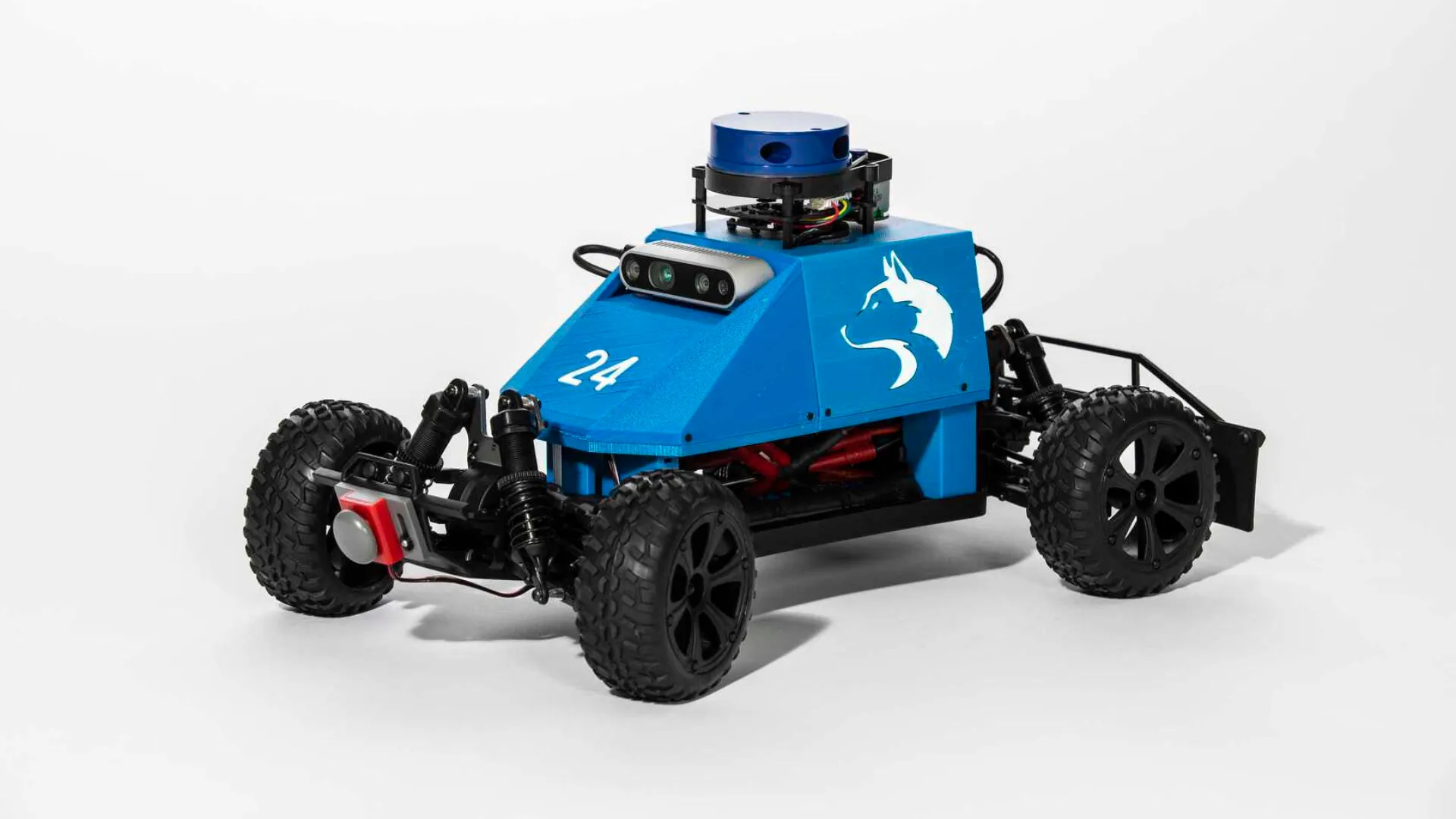
While the bulk of CSE 478 lecture was theoretical, we were able to actually apply that knowledge we had acquired and write in some code for the Mushr crawler. You can learn more about the Mushr platform here.

The important parts of the Mushr platform as it pertained to the class was the 2-d LiDAR mounted to the top of the robot and the Ackerman steering.

The project was split into 3 different parts: localization, control, and planning.

Localization

In this part of the project, we wrote code in order to “track” where the vehicle is in an area with a known map.

Motion Model

The motion model simplifies the car as a bicycle, allow us to take a position & angle $(x,y, \theta)$, wheel angle $(\delta)$, and velocity $(v)$ and predict where it’ll go.

Fig. 1: A diagram demonstrating the points for the kinematic model.

We also add in some stocastic noise to the position, to give some wiggle-room for inaccuracies in any of the ingested data fed to the motion model or account for different environmental conditions.

Sensor Model

To further correct issues with the motion model, we utilize a sensor model (powered by the 2-d LiDAR on top of the Mushr). Utilizing the map for reference, for each point + rotation, we check how different each distance from the LiDAR is from map reference. We once again add stocastic noise to account for small imperfections in the LiDAR.

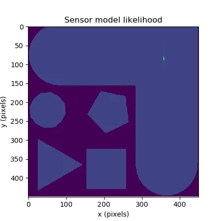Fig. 2: A 2-d heat map showing the most likely positions given certain LiDAR data.

In fusing the sensor and motion models, we are able to get a relatively good idea of where the robot is and isn’t.

Particle Filter

To avoid storing a continous distribution of points, we utilize a particle filter to approximate the potential positions, and then utilize low-variance resampling to ensure we don’t start particles, while also primarily exploring regions of interest.

Control

With an idea of the map and the robot position, we could start controlling the robot and set it along the right planned path. We tested numerous controllers through the project, and landed on PID for controlling wheel speed and steering angle, and Model-Predictive Controller (MPC) to follow a given path.

PID

PID is an extremely simple, and can be expressed with the equation

$$u(t) = - \left(K_p e(t) + K_i \int_0^t e(t')dt' + K_d \frac{de(t)}{dt} \right)$$

Where $K_p$, $K_i$, and $K_d$ are constants, and $e(t)$ is how far the actual value is from the setpoint. Similar to a spring system, we aim to dampen oscillations while avoiding overdampening the system. By changing $K_p$, $K_i$, and $K_d$, we can thus allow for a better response and behavior that matches the setpoint.

MPC

In order to generate the setpoints (which are the steering angle and wheel velocity), we must utilize a planner. While other systems are short sighted and rely on a map, MPC has the ability to weigh different plans and choose the most optimal one. First, it uses a model to solve a $T$-horizon optimization problem against our cost function. This penalizes states and actions that are illegal (colliding with sensed objects or the map walls) or disadvantageous (drifting off course, going slowly) and rewarding speed and following the assigned path. The result is a sequence of actions that minimizes cost. The system does the first action, then repeats the same optimization from its new estimated state, again and again until it arrives at its endpoint.

Planning

In addition to controlling the robot autonomously, we would also need to have it develop its own path, and we did so through a Lazy A* planner.

Halton Sampler

Not unlike the kinematic model, it is impossible to store all of the possible states the robot can be in. As such, we sample the entire map using a detiministic sampler (to avoid variance) to create vertices in the configuration space (the 3 dimensional space that includes the position and rotation of the robot).

In a bog-standard A* implementation, we would create edges to all nearby vertices that don’t collide with the map, but instead, we simply cache vertices that have been explored and solve for the edge when we arrive to them in our path-planning algorithm.

Dubins Path

In order to ensure that paths don’t collide with walls, we utilize the shortest path between the points, which is encapsulated in Dubins paths.

There are six types of Dubins paths:

• LSL, RSR – turning in the same direction

• LSR, RSL – turning in opposite directions

• RLR, LRL – includes a middle turn in the opposite direction

And by checking that at least one of these exists between two vertices, we say that they have a valid edge between them.

Lazy A*

While we could use Djikstra’s to search for an optimal path, it simply is too much work, and can be made more efficient with a fast, efficient heuristic distance from the any vertex and the goal, and adding the accumlated cost-to-come from. That is, we want to find a minimal f-value at any node: $f(n) = g(n) + h(n)$, where $g(n)$ is the cost so far, and $h(n)$ is that heuristic value. With that, we basically do Djistra’s, finding the least cost vertex thus far and exploring from there.

In a bog-standard A* implementation, we would create edges to all nearby vertices that don’t collide with the map when sampling, but instead, we simply cache vertices that have been explored and solve for the edge when we arrive to them in our path-planning algorithm, making the algorithm “lazy”.

Shortcuts

While the Dubin curves are the optimal path between two orientations, we aren’t simply going to each waypoint; rather, we are trying to go from the start position to the end position. As such, we randomly check an amount of the different verticies and see if there’s a direct path between the edges, which is extremely fast compared to doing A* with a large radius between vertices, but still allows us to scan for more “direct” paths between far-apart points.

Conclusion

And with that, we have an autonomous robot that can navigate any space it has a map for, while still avoiding all sorts of obstacles. It was really fun to learn these things, and I learned some things that I would love to implement into personal projects!

As this was a class project, I am not at liberty to share my code publically on the internet; however, if you’d like to see what we cooked up, feel free to contact me.